CSXCAD
Initialization
An openEMS simulation always starts by creating a 3D model of the structure
using the CSXCAD library. All created entities for the simulation are stored
in the csx data structure (or Python object), which must be initialized
first. It’s done by either the InitCSX() method in Matlab/Octave, or
the ContinuousStructure class in Python:
% Matlab/Octave
csx = InitCSX();

# Python
import CSXCAD
csx = CSXCAD.ContinuousStructure()
Once initialized, 3D models can be created by the functions provided by CSXCAD. In Matlab/Octave, nearly all of them accept an old instance of the csx data structure, and returns a modified new one. The Python binding has a more modern coding style in comparison, which achieves this via class methods rather than functions:
% Matlab/Octave
csx = AddExample(csx, arg1, arg2, arg3, ...)

# Python
csx.AddExample(arg1, arg2, arg3, ...)
These CSXCAD functions can be classified into two types, properties and primitives. They define material properties and shapes respectively.
Properties defines the physical property of a material, such as a metal, a thin conducting sheet, a dielectric metarial, a magnetic material. Technically, excitation sources, probes, and field dump boxes are also Properties.
Primitives are the building blocks to create 1D, 2D, 3D shapes, so that one can create simple object such as a Curve, a Polygon, a Box, or a Sphere. More complex structures can be created by combining various primitives. For example, a metal sheet with cylindrical holes can be achieved by combining a metal box with several air cylinders.
See also
See Properties and Primitives for details.
Coordinate Systems
By default, a Cartesian coordinate system is used, which is suitable for most simulations. If the simulated structure is predominantly round, the Cartesian mesh may have a difficult time aligning itself with an object’s surfaces. Hence openEMS provides the alternative cylindrical coordinate system to minimize staircasing errors:
% Matlab/Octave
csx = InitCSX('CoordSystem', '1');

# Python
import CSXCAD
csx = CSXCAD.ContinuousStructure(CoordSystem=1)
Note
This mainly affects meshing of the simulation box during a simulation, not the coordinates of 3D structures themselves. When creating 3D models, their coordinates do follow the meshing coordinate system by default, but it can always be overridden.
Saving
Once modeled, the CSXCAD data structure is usually saved to disk as an
.xml file. It can be inspected by the AppCSXCAD 3D viewer
for debugging:
AppCSXCAD simulation.xml
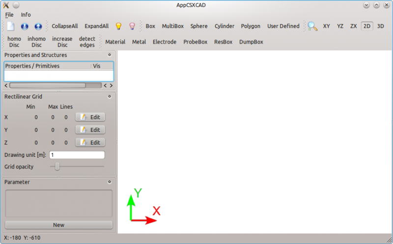
AppCSXCAD, CSXCAD’s official 3D model viewer and editor.
In the Matlab/Octave binding, both the geometry and simulation parameters
are saved together as a self-contained .xml file. The former is
created by InitCSX() and controlled by the csxcad data structure,
the latter is created by InitFDTD() and controlled by the fdtd data
structure. Hence WriteOpenEMS() requires both inputs:
CSX = InitCSX();
FDTD = InitFDTD();

path = '/tmp';
filename = 'simulation.xml';

% write openEMS compatible xml-file
WriteOpenEMS([path '/' filename], fdtd, csx);
In the Python binding, only the CSXCAD geometry information is saved to
the .xml file using the Write2XML()
method:
import pathlib

simdir = pathlib.Path("./")
xmlname = pathlib.Path("simulation.xml")

# concat two paths
xmlpath = simdir / xmlname

csx.Write2XML(str(xmlpath))  # convert Path object to string
Import & Export
Several Matlab/Octave functions are provided to import or export the CSXCAD model to other formats, they include:
-
Especially useful for importing a 3rd-party 3D model (such as a connector).
export_gerber(),export_excellon():CAM file outputs for fabrication. Useful for automated generation of planar circuits.
-
For comparing simulation results with proprietary, commercial tools.
-
For rendering fancy ray-traced 3D images.
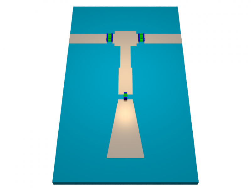
Rendering of a 2.4 GHz planar circuit by raytracing.
Note
Python. These functions are not implemented in Python yet. As
a workaround, for importing, one can use Matlab/Octave to import an
STL model (ImportSTL()), export the result to .xml, and
load the
model in Python via ReadFromXML().
For exporting, AppCSXCAD itself can generate POV-Ray,
STL, X3D, Polydata-VTK, and PNG file formats.
Importing is easy, meshing is hard. Importing an external model is considered an advanced feature, beginners are not recommended to try them before familiarizing themselves with the CSXCAD/openEMS workflow first via basic simulations, as described in First Lessons For Circuit Designers. Creating a meshing-friendly model (see Mesh) is often difficult, so a model and a mesh is usually co-developed. If a model comes from another source, yet the user is not already familiar with the meshing process and its pitfalls, confusing problems may arise.
Models and Simulations Reuse
The development of the Matlab/Octave and Python bindings took different paths, as a result, they behave differently in terms of reusing models and simulations.
Matlab/Octave
The Matlab/Octave binding was written as a pure “XML generator frontend”
to CSXCAD, and the openEMS executable was used as an “executable backend”.
All Matlab/Octave operations (such as geometries and simulation
settings) are only wrapper to the underlying .xml file writer. Once
generated, openEMS is launched and took over the simulation independently.
As a result, the same .xml file can be directly used to replay the same
simulation via the openEMS command-line in the future, even without the
source code. For example, it can be useful for constructing a simulation on
the local machine, but running simulation on a headless server:
openEMS simulation.xml
However, since the Matlab/Octave binding is only an .xml generator without
direct access to CSXCAD itself, the generated .xml file is “a one-way street”
that can’t be reloaded as a Matlab/Octave data structure after the fact.
Source code must be kept if the generated structure or simulation needs any
future modifications. Overall, the Matlab/Octave binding works like a static
website generator. One can generate web pages, but can’t edit the HTML files
back into the source format.
Python
In the Python binding, a decision was made to create a library-level binding to
both CSXCAD and openEMS. When geometries are created, rather than generating the
matching .xml code, it uses the actual funcions and internal data structure
within the CSXCAD library. As a result, it’s possible to reload an existing
CSXCAD 3D .xml model via ReadFromXML().
However, because the simulation is started by invoking openEMS as a library
directly rather than passing simulation parameters via .xml file, no
simulation parameters are written to the file. Hence the file is not standalone
and insufficient to start the simulation. Running the simulation requires a
functional Python script with both an instance of
ContinuousStructure and an instance of openEMS.
However, a sourceless simulation replay is partially possible, by reusing
an earlier CSXCAD 3D .xml model via ReadFromXML()
and setting up the rest.
If there’s a need, in principle one can write a self-written lightweight wrapper
for this purpose (no built-in implementations exist currently)
Note
Replaying Simulations. Sometimes it may be desirable to “replay” an existing simulation setup without access to the Matlab/Octave or Python source code. This is possible in Matlab/Octave, but only partially possible in Python.
Post-Processing. In all cases, post-processing simulation results
always requires source code. The program openEMS itself is only a
field solver engine. For analysis, we rely on Matlab/Octave or Python
routines.
Third-Party Apps. If you’re developing a third-party simulator
or binding based on openEMS, it’s recommended to generate a simulation
.xml and to call openEMS as an executable. The openEMS is a shared
library, but it’s so far not designed for public use. On the other
hand, the CSXCAD library is designed to be publicly reusable, so it’s
acceptable to either generate the .xml yourself or invoke the CSXCAD
library to do that, as a result, the recommendation is a hybrid of
the approaches used by Matlab/Octave and Python bindings.
Modeling via a GUI?
In principle, it’s feasible to make or tweak a 3D model using the
AppCSXCAD GUI. Geometries and mesh lines can be added
by the GUI (or an initial program), a modified version can be saved
and read into Python later for simulation via
ReadFromXML().
This method circumvents programmatic modeling
(as decribed in Primitives) entirely - although it
has not been put in use by anyone to our best knowledge.
On the other hand, there are numerious attempts over the years to create models using GUI-based or high-level tools, to varying degrees of success.
The first general idea is to create the structure first in a
general-purpose CAD like FreeCAD. This can then be exported as
a 3D model and be loaded into CSXCAD via ImportSTL() for
simulation. By editing the CSXCAD object further, ports and
probes can also be modeled as a GUI.
The second general idea, specific to planar circuits and circuit board simulations, is to first create the circuit board using an EDA tool such as gEDA, pcb-rnd, or KiCad. The circuit layout can then be exported as a 2D vector image format, such as HyperLynx, Gerber, SVG or PDF. The polygons in these images are then extracted and imported as CSXCAD polygons.
The third general idea, is to create a high-level programming library for defining high-level objects such as traces, vias, circuit board layers, so that they can be created one object at a them, rather than one polygon at a time.
Important
Third-Party Tools. These tools are developed by third parties, and not officially supported by the openEMS project. Most of them are highly experimental and incomplete. They’re described here for completeness. The project forum is also open to the discussions of their uses.
Importing is easy, simulation is hard. These tools should be considered advanced applications. Beginners are not recommended to try them before familiarizing themselves with the CSXCAD/openEMS workflow first via basic simulations, as described in First Lessons For Circuit Designers. Trying to import a circuit board without understanding the concept of ports, boundary conditions or meshing rules leads to failures, especially when most of these tools are highly experimental and incomplete.
Don’t work in isolation. By far there are already 7 different tools that attempt to automate modeling of circuit boards and 3D objects for openEMS. Instead of creating another one from scratch, it’s probably a good idea to have a discussion with the authors of these existing tools.
Examples of these tools include:
FreeCAD-OpenEMS-Export, developed by Lubomir Jagos.
FreeCAD-based model and port edits, with CSXCAD export.
IntuitionRF, developed by Juleinn.
It allows one to mesh structures interactively via Blender.
pcb2csx, developed by Evan Foss.
It’s a plugin to the EDA tool pcb-rnd, allowing one to export an existing circuit board layout to CSXCAD.
http://repo.hu/cgi-bin/pool.cgi?project=pcb-rnd&cmd=show&node=s_param
gerber2ems, developed by Antmicro.
It allows one to export an existing PCB layout as a Gerber file, which can then be converted and imported as a CSXCAD model.
pcbmodelgen, developed by jcyrax.
It converts a KiCad layout file into the CSXCAD model, also with experimental auto-meshing support.
pyems, developed by Matt Huszagh.
It’s a high-level Python interface to openEMS, which allows the programmatic creation of high-level structures such as circuit boards, traces, vias, PCB layers. It has also an experimental auto-mesh generation algorithm.
hyp2mat, developed by Koen De Vleeschauwer and distributed officially as part of openEMS.
It converts a HyperLynx layout file (can be generated by PCB EDA tools, including EAGLE or KiCad 6). The geometries are extracted to generate an Octave script with commands to create the CSXCAD model.
In principle, it can be used with Python as well, by exporting the model to XML in Octave via
WriteOpenEMS(), and importing the model viaReadFromXML(). But no one has tested it.Currently it’s retired and no longer maintained.
Note
The old project wiki also described this following idea to convert circuit board layouts from Gerber, PDF, DXF, or G into CSXCAD models. This idea may be of interest to developers working on automated CSXCAD model generation.
PCB layers in Gerber files can be converted to PDF by means of gerber2pdf which can be found on Sourceforge (editor’s note: native PDF, SVG and DXF exports are available in many EDA packages). The PDF can be imported into Inkscape just as it is the case for DXF files. Within Inkscape, the usually closed paths can be modified (either manually or with filters) such that they result in a suitable list of polygon nodes for openEMS.
Sometimes these polygons or curves have too many nodes. The number of nodes can be reduced with the Inkscape function “Path” > “Simplify”. The amount of reduction is controlled by the parameter “Simplification Threshold” which can be found under “Preferences” > “Behavior”. These paths are still Bézier curves which must be converted into polygons. This is achieved with “Extensions” > “Modify Path” > “Flatten Béziers”. The parameter in this dialog also controls the number of resulting points.
When all nodes are as required, the paths can be exported as a HTML5 Canvas. The resulting file can then be processed with an ASCII Editor. The numbers after the moveTo and lineTo statements are the polygon nodes X- and Y- coordinates respectively. However, they still must be transformed ba a liner transform given in the transform statement. The first four numbers a matrix by which the node coordinates have to be multiplied and the remaining two numbers are a vector which has to be added.
The result will be the node coordinates in HTML pixels with X counting from left to right and Y counting from top to bottom, which does not conform to the coordinate system of the Inkscape canvas.
In order to have the same axes as in Inkscape (X left to right and Y bottom to top), the fourth an sixth number have to be multiplied by -1 and the image height has to be added to the sixth number. Now the coordinates are in the usual coordinate system but still in HTML5 pixels. The ratio of pixels to mm or other units of length can finally be found under the document properties in Inkscape. This factor can be applied in Octave/Matlab. This finally gives polygons which can be processed by openEMS.